It’s been almost 9 years since the introduction of SmokeFree legislation in the UK (although we elves still return from a night out smelling of campfire smoke). However, secondhand smoke is still accountable for 600,000 deaths annually.
Smoke free policies can be implemented at the micro-level (i.e. the individual level or in homes), the meso-level (i.e. in organisations, such as public healthcare facilities, higher education centres and prisons) or the macro-level (i.e. in an entire country). In many countries, smokefree legislation is at the macro-level, although exemptions exist at the meso-level. For example, in the UK, specific rooms in prisons and care homes are exempt from this legislation.
In their Cochrane review, Frazer and colleagues review the evidence for meso-level smoking bans (in venues not typically included in smokefree legislation) on 1) passive smoke exposure, 2) other health-related outcomes and 3) active smoking, including tobacco consumption and smoking prevalence.

Worldwide, secondhand smoke is still accountable for 600,000 deaths annually.
Methods
Identification of included studies
The authors searched online databases of clinical trials, reference lists of identified studies and contacted authors to identify ongoing studies. Studies were included if they:
- Were conducted from 2005 onwards;
- Were conducted in public healthcare, higher educational or correctional facilities (i.e. prisons or military institutions);
- Assessed the impact of either partial or complete bans;
- Had a minimum of 6 months follow-up for measures of smoking behaviour;
- Were quasi-experimental (i.e. controlled before-and-after studies), interrupted time series or uncontrolled before-and-after studies);
- Assessed the impact of tobacco bans or policies on either the:
- Primary outcomes: reducing secondhand smoke exposure or otherhealth outcomes; or
- Secondary outcomes: tobacco consumption and smoking prevalence.
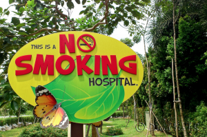
The introduction of smoking bans in psychiatric hospitals and prisons is extremely controversial.
Results
Characteristics of included studies
No randomised controlled trials (RCTs) were found. 17 observational studies were identified (three using a controlled before-and-after design with another site for comparison and 14 using an uncontrolled before-and-after design). Of these 17 studies:
- 12 were based in hospitals;
- 3 in prisons;
- 2 in universities.
Five studies investigated the impact of smoking bans on two participant groups (i.e. staff and either patients or prisoners).
The 17 studies were conducted in 8 countries: the USA (6 studies), Spain (3 studies), Switzerland (3 studies), Australia, Canada, Croatia, Ireland and Japan (all 1 study). Eight of these were conducted in US states or countries with macro-level (i.e. national) smoke-free legislation, eight with no legislative bans and one which compared all 50 US states (some with national bans and others without).
Main findings
There was considerable heterogeneity between the 17 studies and so a meta-analysis of all studies was not conducted. Instead studies were analysed using aqualitative narrative synthesis according to each of the outcome measures:
Reducing secondhand smoke exposure
Four studies assessed secondhand smoke exposure, finding that a reduction in exposure was observed in all three settings after smoking bans. However, none of the studies in the review used a biochemically validated measure of smoke exposure such as cotinine or carbon monoxide levels.
Other health outcomes
Four studies examined the impact of partial or complete smoking bans on health outcomes including smoking-related mortality. Two were conducted in prisons, one in a hospital and one in a secure mental hospital (Etter et al, 2007). All of these studies observed improvements in smoking-related morbidity and mortality after smoking bans. One of these assessed the impact of smoking bans in prisons in all 50 US states and found that smoking-related mortality was reduced in those prisons that had a smoking ban for more than 9 years.
Tobacco consumption and smoking prevalence
Thirteen studies reported data on the effect of smoking bans on smoking prevalence and five of these reported data on two populations within settings (i.e. prisoners and prison staff).
Eleven of these studies were included in a meta-analysis (using the Mantel-Haenszel fixed-effect method) and the data from the 12,485 participants in these studies was pooled. Although there was considerable heterogeneity between these studies (I2 = 72%; where a higher I2 value is evidence of higher levels of heterogeneity), this heterogeneity was lower within subgroups (e.g. in prisoners or hospital staff).
Ten studies conducted in hospital settings found mixed evidence for the impact of smoking bans on smoking prevalence. Eight of these studies were included in the meta-analysis and there was evidence that smoking bans reduced active smoking rates among hospital staff (risk ratio (RR) 0.71, 95% confidence interval (CI) 0.64 to 0.78, n = 4,544, I2 = 76%) and patients (RR 0.84, CI 0.76 to 0.98, n = 1442, I2 = 20%).
The one study in a prison setting found no evidence of a change in smoking prevalence among staff or prisoners after a smoking ban (RR 0.99, CI 0.84 to 1.16, n = 130).
Two studies in university settings observed reductions in smoking prevalence after smoking bans (RR 0.72, CI 0.64 to 0.80, n = 6,369, I2 = 59%), although one study only observed this among male ‘frequent’ smokers.
Quality of the evidence
The evidence was judged to be of low quality as all of the studies wereobservational (none used a RCT design) and the risk of bias was rated as high.

Banning smoking in hospitals and universities increased the number of smoking quit attempts and reduced the number of people smoking.
Conclusion
Overall, this review finds evidence of smoking bans on:
- reducing smoking prevalence in hospitals and universities, with the greatest reductions among hospital staff;
- reduced mortality and exposure to secondhand smoke in hospitals, universities and prisons.
Limitations
The quality of the evidence was low and the authors conclude that ‘we therefore need more robust studies assessing evidence for smoking bans and policies in these important specialist settings’. Limitations with the studies included in the review include: small sample sizes in some studies, a lack of a control location for comparison in all but three studies and a high level of heterogeneity between and within the different settings (e.g. the hospital settings included a cancer hospital, psychiatric hospitals and general hospitals).

We need more robust studies assessing the evidence for smoking bans and policies in specialist settings.
Discussion
The authors report that given this evidence, smoking bans at the meso-level should be considered as part of multifactorial tobacco control activities to reduce secondhand smoke exposure and smoking prevalence.
Given that the introduction of these bans particularly in psychiatric hospitals and prisons is controversial, the introduction of these bans should be sensitive to the needs of populations. For example, bans in psychiatric hospitals should be implemented in consultation with psychiatrists to ensure that the improved health outcomes of patients is considered first and foremost. As the evidence is currently weak, with a high risk of bias, any interventions should be closely monitored.
More robust studies are needed, using a control group for comparison, assessing smoke exposure using biochemically validated measures, using long-term follow-ups of at least 6 months and reporting smoking prevalence both before and after the introduction of the ban.

It is not possible to draw firm conclusions about institutional smoking bans from the current evidence.
Links
Primary paper
Frazer K, McHugh J, Callinan JE, Kelleher C. (2016) Impact of institutional smoking bans on reducing harms and secondhand smoke exposure. Cochrane Database of Systematic Reviews 2016, Issue 5. Art. No.: CD011856. DOI: 10.1002/14651858.CD011856.pub2.
Other references
, . (2007) Acceptability and impact of a partial smoking ban in a psychiatric hospital.. Preventive Medicine 2007;44(1):64–9. [PubMed abstract]